As someone who has been involved in the world of word vectors since 2007, it’s been fascinating to watch the innovative applications that they’ve been put to over the last few years. After reading Ryan Heuser’s ‘Word Vectors in the Eighteenth Century, Part 1,’ I was left impressed not only by the thoughtful scholarship but also by the sheer mystery of how such an unusual analogy (“riches are to virtue as learning is to genius”) might be encoded in the lexical statistics of a corpus of eighteenth-century texts (ECCO-TCP). This post is an attempt to answer that question for myself. My discoveries along the way may be of interest to others curious about the lexical contexts of ‘virtue,’ ‘riches,’ ‘learning,’ and ‘genius’ in the eighteenth century, or to anyone who finds themselves in the business of interpreting word vectors.
Very good descriptions of word vectors and vector space models have been provided by others inside and outside of the digital humanities, but they’re still unknown enough within DH that I thought it might be worth giving a brief overview and history. If you’re already familiar with the mechanics and history of vector space models and want to get straight to the investigation of virtue, riches, learning, and genius in ECCO-TCP, feel free to skip ahead.
Lexical maths and fresh politeness
A vector is simply an ordered list of numbers. The vectors in a vector space model need not necessarily represent words, but for the models that interest us here, every word is assigned a unique vector that contains information about the lexical contexts in which it appears in a large body of text. There are many different ways in which this information can be encoded. Here’s one particularly simplistic approach: Start by creating a vector that that is intended to represent the contextual usage of a particular word (the so-called target word) in some particular corpus, denoted here by V(target). Let each component of that vector correspond to a different context word that appears in the same sentence as the target word, and instantiate that component with the number of sentences in which the two words co-occur. Suppose our target word is king, and our context words are he, his, him, she, her, hers, crown, throne, royal, and majesty. The resulting ten-dimensional vector might look something like this:
| he | his | him | she | her | hers | crown | throne | royal | majesty |
| 6509 | 8612 | 3093 | 486 | 1053 | 1 | 360 | 223 | 335 | 491 |
In other words, king appears in the same sentence as he 6509 times, in the same sentence as his 8612 times, and so on. A handy thing about vectors is that we can do arithmetic with them. For example, if we assume the following plausible vector for the target word man…
| he | his | him | she | her | hers | crown | throne | royal | majesty |
| 10438 | 10466 | 3409 | 1582 | 1961 | 12 | 70 | 31 | 42 | 49 |
…we can calculate what we get if we subtract V(man) from V(king), by taking the difference between corresponding components:
| he | his | him | she | her | hers | crown | throne | royal | majesty |
| -3929 | -1854 | -316 | -1096 | -908 | -11 | 290 | 192 | 293 | 442 |
Not surprisingly, we end up with a vector V(king) – V(man) that has low values for words that appear more frequently with man than with king, and higher values for words that appear more frequently with king than with man. There are some obvious problems with vectors that have been constructed in this way. For one thing, we’re not controlling for the frequency of the target words. A relatively rare word like Croesus might yield a vector of very small numbers across the board. So although we might hope that V(king) – V(Croesus) would yield a vector that could tell us something about the differences between the discourse contexts of king and Croesus, in actuality we’d likely get a vector that is nearly identical to king’s, which would not be particularly useful. And we’re not controlling for the frequency of context words, so common words like he, his, and so on will have undue influence. Even so, if we continue the thought experiment by adding V(woman) to V(king) – V(man), it’s plausible that we’d get something like the following:
| he | his | him | she | her | hers | crown | throne | royal | majesty |
| -2680 | -1003 | -4 | 701 | 1698 | 19 | 306 | 196 | 301 | 448 |
In other words, we’d get a vector that has low values for context words which we expect man and king to share in common (e.g. he, his, him), high values for context words with which woman occurs much more frequently than man (e.g. she, her, hers), and high values for context words with which king occurs much more frequently than man (e.g. crown, throne, royal, majesty). These are all properties that we’d expect V(queen) to have. If we’re lucky, it’s even possible that V(queen) would come up as the best match if we were to quantify the overall similarity of V(king) – V(man) + V(woman) to the vectors of every possible target word in our corpus. If this turned out to be true, then this vector space model could be said to have successfully completed the analogy “man is to king as woman is to ___.”
The above example is not a particularly good one except for illustrative purposes, because of how naïve this particular algorithm for building a vector space model is. Not only does it fail to control for word frequency, it only attends to ten context words that we cherry-picked rather than the thousands of different words that appear in our corpus. This model is not likely to do well on any battery of analogy questions. However, I include the example because I hope it’s intuitive to readers who aren’t intimately familiar with these models, and also to underscore that it’s possible to do analogical vector arithmetic in fairly traditional vector spaces, even though this sort of thing has become much more closely associated with popular recent tools such as word2vec, which construct a rather different sort of vector that I’ll describe shortly. Indeed, Levy, Goldberg, & Dagan (2015) have demonstrated that traditional count-based models can hold their own on analogy tasks against word2vec, with the requisite tweaks.
A historical aside: Vector space models have a long history in computational linguistics, information retrieval, and cognitive science. One interesting predecessor in the world of cognitive psychology was the famed psychologist Charles Osgood’s semantic differential, an experimental technique in which study participants had to rate words on dimensions such as active versus passive, angular versus rounded, and small versus large. On a scale of fresh to stale, how fresh (stale) is the concept POLITE? (Empirical answer below.)
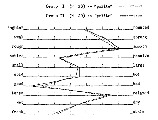
Semantic differentials, averaged across two groups of twenty study participants each. From The Nature and Measurement of Meaning, pp. 229. Psychological Bulletin, 49(3), May 1952.
Tasks to which vector space models have been applied include retrieving documents related to a particular search query, grouping together documents with related meanings, classifying texts by genre, essay grading, modelling how the human brain might represent some aspects of lexical semantics, and many others. As a result, much attention has been paid to building models that optimize performance on various evaluation criteria, such as maximizing correlations with human judgments of word similarity, scores on multiple-choice tests of synonymy, or accuracy on sentence completion tasks. Less attention has been paid to questions of interpretation that are more relevant to the humanities (how best to interpret the dimensions of various species of word vector, what kinds of information can and cannot be retrieved from the statistics of language, what kinds of analogies are most and least successfully represented in vector spaces, etc.), although there has been important research in all of these areas as well.
Vector space models for which the initial step is to count the number of contexts (sentences, documents, etc.) in which context words co-occur with the target word are generally called count-based models; these can be viewed as upgraded versions of the naïve model illustrated earlier in this post. These are generally made more robust by incorporating transformations that control for overall word frequency and/or make the model more robust to data sparsity. It’s also common for count-based models to use alternative notions of the ‘context’ of a target word, such as a ‘window’ that includes only a small number of terms that appear just to its left or right.
In some count-based models, the dimensions correspond directly to transformed counts of particular words (e.g., Bullinaria & Levy 2007), whereas others use statistical methods to transform high-dimensional vectors to lower-dimensional versions (Landauer & Dumais 1997; Pennington, Socher, & Manning 2014), making the interpretation of individual dimensions a bit more fraught. Depending on who you ask, the class of ‘count-based models’ may or may not include random vector models (Jones, Willits, & Dennis, 2015) such as random indexing (Kanerva, Kristofersson, & Holst 2000; Sahlgren 2005) and BEAGLE (Jones, Kintsch, & Mewhort, 2006), which assign a randomly initialized and unchanging index vector to each context word, and an initially empty memory vector to each target word. As the algorithm chugs through a corpus of texts, the index vectors of words that appear in the context of a target word are added to the target word’s memory vector. Ultimately, memory vectors that repeatedly have the same index vectors added to them (crown, throne, royal, majesty) end up more similar to each other, resulting once again in a space of memory vectors in which words that appear in similar contexts end up having similar vectorial representations.
An example of how vector similarity between vectors representing a word and the word’s context changes with context in a random vector model. From Jones & Mewhort (2007), Psychological Review, 114(1), p. 18.
Count-based models are frequently contrasted with prediction-based[1] models, such as those generated by the popular software package word2vec (Mikolov, Chen, Corrado, & Dean, 2013). I won’t explain the inner workings of word2vec in detail as this has been done by many others, other than to say that word2vec consists of two distinct algorithms. The first, continuous bag of words (CBOW), attempts to predict the target word given its context, while the skip-gram algorithm attempts to predict a word’s context given the word itself. Skip-grams seem to achieve equal or superior performance to CBOW for most purposes, and as such this is the algorithm employed most frequently in the literature. To optimize its ability to predict contexts that actually appear in the corpus, and to minimize its tendency to predict contexts that don’t, the algorithm continuously tweaks a large number of parameters according to a partially stochastic process. Ultimately, the learned model parameters corresponding to a given target word are treated as that word’s vector representation. These relatively low-dimensional [2] vectors are often described as “word embeddings,” to distinguish them from vectors of models in which every dimension corresponds to one of an extremely large number of context words.
Levy & Goldberg rocked the world of word embeddings in 2014 when they demonstrated that despite the apparent gulf between the inner workings of prediction-based and count-based models, word2vec’s skip-gram algorithm is implicitly factorizing a word-context PMI matrix. In other words, the core of what it’s doing, mathematically speaking, is not much different than the sort of thing that some count-based models have been doing for awhile. This is particularly clear in the case of the Glove model (Pennington, Socher, & Manning, 2014), which explicitly factorizes a word-context PMI matrix, and generally achieves comparable results to word2vec. However, word2vec has two other properties that contribute to its continued popularity:
- There is a very good, fast implementation available from Google at https://code.google.com/archive/p/word2vec/ which runs easily on a laptop with limited memory, and an excellent Python implementation available from Radim Řehůřek.
- Compared against several alternatives, it works quite well “off the shelf” with the default settings, as recently demonstrated by Pereira et al. (2016).
Given this combination of ease of use and state-of-the-art performance, it’s no surprise that researchers have been using word2vec for everything from sentiment classification (Xue, Fu, & Shaobin, 2014), to experimental deformation of Pride and Prejudice (Cherny, 2014), to predicting relationships between smell-related words using a combination of linguistic and olfactory data (Kiela, Bulat & Clark 2015). In the sections that follow, I wanted to follow up on Ryan Heuser’s use of word2vec to investigate the contexts of ‘virtue,’ ‘learning,’ ‘riches,’ and ‘genius’ within the eighteenth-century corpus ECCO-TCP. In the words of 21st century Internet media company and clickbait purveyor BuzzFeed.com (2016), “the answer may surprise you.”
A sceptical interlude
So far, we’ve strongly suggested that these analogical arithmetic problems work in vector space models for exactly the reason you’d think they should. If A is to B as C is to D, then the conceptual difference between D and C should be approximately equal to the conceptual difference between B and A. Or to say the same thing in terms of vectors,
V(woman) – V(man) ≈ V(queen) – V(king)
and, rearranging the terms algebraically,
V(king) – V(man) + V(woman) ≈ V(queen)
which is the very proposition we tested in the illustrative example that we stepped through earlier. But what if the reason this works has nothing to do with the analogical relationship between king/queen and man/woman, but is rather due solely to the fact that the contexts in which queen is found share lexical material with contexts in which king and woman tend to appear? On this view, the presence of man is irrelevant, and we should expect V(king) + V(woman) to yield a vector that is even more similar to V(queen) than the needlessly complex V(king) – V(man) + V(woman).
How would we test this hypothesis? As previously implied, the canonical test for whether a vector space model can correctly complete the analogy “A is to B as C is to __” is to consider the vectors of all the different target words in our model, and to sort them by their degree of similarity to V(C) – V(A) + V(B). If the word corresponding to the correct answer is on top (or near the top, if our criterion for success is a little looser), then we declare success and move on.
But, sceptics that we are, we don’t just want to compare V(queen) to V(king) – V(man) + V(woman); we also want to compare it directly to V(king) + V(woman). If it’s more similar to the latter than to the former, then that’s evidence that our vector space model hasn’t picked up on an analogical relationship, but rather a combinatorial one: that is, that the discourse contexts of queen share lexical material with those of king and woman, and the lexical context of man is largely irrelevant.
Let’s test whether this is true in ECCO-TCP. Because the word2vec algorithms involve a stochastic component, I created six models from ECCO-TCP using Google’s code, using the skip-gram algorithm with the default window size (5 words on either side of the target). Just as Mikolov et al. reported in their original paper using the Google News corpus, computing V(king) – V(man) + V(woman) in ECCO-TCP yields a vector closer to the vector of the target word V(queen) than any other. Here are the ten most similar vectors to V(king) – V(man) + V(woman) in each of the six models, using the vector cosine as the similarity function:
Most similar vectors to V(king) – V(man) + V(woman)
| Model 1 | Model 2 | Model 3 | |||
| 0.8428452 | queen | 0.8482416 | queen | 0.8460983 | queen |
| 0.8044825 | king | 0.7945445 | king | 0.8085347 | king |
| 0.7614051 | princess | 0.7806808 | princess | 0.7889509 | princess |
| 0.6964183 | berengaria | 0.7120882 | adelais | 0.7216414 | ethelburga |
| 0.6949631 | adelais | 0.7057881 | archduchess | 0.7086453 | berengaria |
| 0.6942522 | infanta | 0.7038351 | ethelburga | 0.7041441 | elizabeth |
| 0.6883563 | elizabeth | 0.7000595 | atheling | 0.7023171 | anjou |
| 0.6814717 | ethelburga | 0.6953432 | infant | 0.7022427 | infanta |
| 0.6765546 | maude | 0.6914362 | berengaria | 0.702105 | atheling |
| 0.6713672 | mary | 0.6906615 | maude | 0.7013055 | adelais |
| Model 4 | Model 5 | Model 6 | |||
| 0.8556742 | queen | 0.8349165 | queen | 0.8482416 | queen |
| 0.8013376 | princess | 0.7957921 | king | 0.7945445 | king |
| 0.8002654 | king | 0.7841321 | princess | 0.7806808 | princess |
| 0.7235335 | infanta | 0.7190303 | ethelburga | 0.7120882 | adelais |
| 0.6992922 | archduke | 0.7120405 | infant | 0.7057881 | archduchess |
| 0.6983816 | boleyn | 0.7108373 | berengaria | 0.7038351 | ethelburga |
| 0.6973003 | anjou | 0.7077445 | atheling | 0.7000595 | atheling |
| 0.6860953 | berengaria | 0.7030088 | adelais | 0.6953432 | infanta |
| 0.6837387 | empress | 0.697409 | ethelred | 0.6914362 | berengaria |
| 0.6816853 | adelais | 0.6963173 | elizabeth | 0.6906615 | maude |
Sure enough, ‘queen’ tops the list in every instance. To continue with our original plan, what do we find when we look for the most similar vectors to V(king) + V(woman)? That turns out to yield the following:
Most similar vectors to V(king) + V(woman)
| Model 1 | Model 2 | Model 3 | |||
| 0.8015435 | king | 0.8013967 | king | 0.8045057 | king |
| 0.7678058 | queen | 0.7652432 | queen | 0.7655054 | queen |
| 0.741822 | woman | 0.7480951 | woman | 0.7540007 | princess |
| 0.741563 | princess | 0.7397602 | princess | 0.7470537 | woman |
| 0.7386138 | emperess | 0.7268931 | monarch | 0.7259848 | prince |
| 0.7283809 | prince | 0.7170094 | prince | 0.7146243 | man |
| 0.7053233 | man | 0.7058172 | man | 0.7020829 | emperess |
| 0.7038987 | monarch | 0.7048363 | nobleman | 0.7010611 | monarch |
| 0.7034665 | nobleman | 0.6988204 | potiphar | 0.7009223 | nobleman |
| 0.6957511 | rizio | 0.6987603 | emperess | 0.6943904 | hephoestion |
| Model 4 | Model 5 | Model 6 | |||
| 0.7972889 | woman | 0.7975317 | king | 0.8041995 | king |
| 0.7931416 | king | 0.7555078 | queen | 0.7609213 | queen |
| 0.7569074 | queen | 0.7445927 | princess | 0.7521903 | woman |
| 0.748388 | princess | 0.7422349 | woman | 0.7455949 | princess |
| 0.736528 | man | 0.7217866 | prince | 0.7344416 | prince |
| 0.7338801 | husband | 0.7178928 | emperess | 0.7165893 | nobleman |
| 0.718644 | prince | 0.7142186 | nobleman | 0.7152176 | man |
| 0.7119973 | monarch | 0.7104293 | man | 0.7125439 | husband |
| 0.7093402 | lover | 0.7009807 | hephoestion | 0.7089317 | monarch |
| 0.7019279 | dorastus | 0.6977934 | lucumon | 0.7017831 | lucumon |
This is an anticlimactic but reassuring result: V(queen)’s similarity to V(king) – V(man) + V(woman) is reliably slightly greater than its similarity to V(king) + V(woman), in absolute numerical terms as well as relative to other words. Removing what is contextually shared by king and man and adding the result to woman yields a better match to queen than merely combining what is common to king and woman. In other words, the lexical statistics of king, queen, man, and woman contain analogical, not just combinatorial, information.
What is genius?
The investigation that follows was prompted by my curiosity surrounding Ryan Heuser’s investigation of the analogy “riches is to virtue as learning is to genius” in Edward Young’s Conjectures on Original Composition. Young explains his reasoning as follows:“If I might speak farther of learning, and genius, I would compare genius to virtue, and learning to riches. As riches are most wanted where there is least virtue; so learning where there is least genius. As virtue without much riches can give happiness, so genius without much learning can give renown.”
Should we then expect to find that V(virtue) – V(riches) + V(learning) ≈ V(genius), just as V(king) – V(man) + V(woman) ≈ V(queen)? Intuitively, this seems like a lot to expect from a vector space model. I’m not sure that most individuals, either today or in the 18C, would immediately complete the analogy “riches is to virtue as learning is to ____” with genius. It’s also not clear exactly how or why we should expect this parallel to manifest itself in the statistics of language, whereas with king, man, woman, and queen it’s a bit more obvious (as I argue above). But the math seems to work, more or less: Ryan finds that out of the 129,098 word vectors in his model, V(genius) is the sixth most similar to V(virtue) – V(riches) + V(learning)! In my own six word2vec models, V(genius) has a median rank of 14th most similar (likely owing to differences in our corpus preprocessing, algorithm implementation, measures of vector similarity, and/or random variation)—a little lower than in Ryan’s model, but still holding its own against tens of thousands of alternatives.
What could account for this? As Ryan points out, there is another important symmetry in the relationship between riches/virtue and learning/genius: Both virtue and genius express “ethically immanent and comparatively individualist forms of value,” whereas learning and riches express “more socially-embedded and class-based forms of value.” If that is reflected in the linguistic contexts in which each of these words occur in ECCO-TCP, we might expect that the latter would ‘cancel out’ in the – V(riches) + V(learning) part of the formula V(virtue) – V(riches) + V(learning), leaving virtue to be combined with aspects of learning that are free of whatever overtones that learning and riches might share.
But is that the only possibility? There are other potential explanations. For example, could it be that the discourse contexts in which genius appears are just really similar to the contexts in which learning appears, and that V(virtue) and V(riches) are just introducing noise? Or that the similarity of V(genius) to V(learning) + V(virtue) (or to V(virtue) – V(riches), or to V(learning) – V(riches)) is the underlying cause of the finding that V(virtue) – V(riches) + V(learning) ≈ V(genius)?
Given the build-up in the previous section, you can probably see where this is headed. In my own six word2vec models, V(learning) + V(virtue) is even more similar to V(genius) than is V(virtue) – V(riches) + V(learning), having a median rank of 6 and median cosine similarity of .767:
Most similar vectors to V(learning) + V(virtue)
| Model 1 | Model 2 | Model 3 | |||
| 0.8989632 | learning | 0.8990331 | learning | 0.9003327 | learning |
| 0.862316 | virtue | 0.8639017 | virtue | 0.865199 | virtue |
| 0.7992792 | piety | 0.8079271 | piety | 0.804012 | piety |
| 0.7816411 | science | 0.7708147 | probity | 0.7795218 | science |
| 0.7774129 | genius | 0.769802 | science | 0.7786523 | probity |
| 0.7764739 | wisdom | 0.7687995 | genius | 0.7729051 | wisdom |
| 0.763268 | probity | 0.7681421 | wisdom | 0.7707377 | genius |
| 0.7384178 | knowledge | 0.7445111 | integrity | 0.7378831 | knowledge |
| 0.7366986 | philosophy | 0.7346854 | morals | 0.7342591 | morality |
| 0.7346987 | morality | 0.7289329 | erudition | 0.7320021 | integrity |
| Model 4 | Model 5 | Model 6 | |||
| 0.901885 | learning | 0.9010782 | learning | 0.897611 | learning |
| 0.8747023 | virtue | 0.8701212 | virtue | 0.8649616 | virtue |
| 0.7941153 | piety | 0.7893927 | piety | 0.7979715 | piety |
| 0.7817841 | probity | 0.7749184 | science | 0.7828707 | probity |
| 0.7657776 | wisdom | 0.7683302 | probity | 0.7820131 | science |
| 0.7628907 | genius | 0.766835 | wisdom | 0.7652096 | genius |
| 0.7628165 | science | 0.7531987 | genius | 0.7627894 | wisdom |
| 0.7384895 | erudition | 0.7428998 | morality | 0.7471387 | knowledge |
| 0.7359856 | knowledge | 0.741063 | integrity | 0.7411712 | morality |
| 0.7331604 | unblemished | 0.74005 | knowledge | 0.7368826 | erudition |
V(genius) was not at all similar to V(virtue) – V(riches) nor to V(learning) – V(riches). It was moderately similar to V(learning) alone, but not as much so as to V(virtue) + V(learning).
To recap: Across six word2vec models of ECCO-TCP that varied only in the element of random change inherent in the skip-gram algorithm itself, V(genius) was more similar to V(learning) + V(virtue) (median rank = 6, cos = .767) than it was to V(virtue) – V(riches) + V(learning) (median rank 14, cos = .591) or to V(learning) alone (median rank = 10, cos = .726). These differences appear to be statistically significant[3]. In Ryan’s word2vec model, V(genius) has a cosine similarity of .779 to V(learning) + V(virtue), .651 to V(virtue) – V(riches) + V(learning), and .731 to V(learning)—the same ordinal pattern of effects.
None of this should be taken as a claim that the concept genius was merely a virtue-infused notion of learning, nor as any sort of claim that the complex constellation of ideas that surrounded genius can or should be distilled to a simple story. Entire books have been written on the incredible array of uses to which the term has been put, such as Ann Jefferson’s Genius in France and Darrin McMahon’s Divine Fury: A History of Genius. As Jefferson notes, it would be misleading to assume a strong cultural consensus around the term at all in the 18C, as different authors described it as something to be admired and something to be suspicious of, as something to be emulated and as something incapable of emulation, as something vigorous and vital and as something aberrant or even sickly. Aside from the varying connotations and functions of the term, its very meaning was exceedingly labile, as Carson (2016) relates in this description of its mentions in reference materials of the time:
“With regard to the meaning of ‘genius,’ there was a range of possibilities, as Samuel Johnson makes clear in his Dictionary of the English Language (1755). ‘Genius’ could signify a spirit (‘the protecting or ruling power of men, places, or things,’ as Jonson put it); ‘a man endowed with superior faculties’; ‘mental power or faculties’ themselves; a natural disposition ‘for some peculiar employment’; or nature or disposition broadly understood, such as ‘the genius of the times’ or, very commonly, the genius of a people. The Encyclopaedia Britannica of 1771 also defined ‘genius’ first as ‘good or evil spirit,’ and then as ‘a natural talent or disposition to do one thing more than another,’ emphasizing with the latter that ‘art and industry add much to natural endowments, but cannot supply them where they are wanting.’”
John Carson, Genealogies of Genius, p. 50
No vector space model will give us anything close to a complete understanding of this multifaceted term. Yet if we were forced to come up with a handful of terms such that the combination of their 18C discourse contexts was similar to the lexical contexts in which ‘genius’ appeared, we could do worse than to look at the words with the most similar vectors to genius in ECCO-TCP:
Most similar vectors to V(genius)
| Model 1 | Model 2 | Model 3 | |||
| 0.7910758 | talents | 0.7824867 | talents | 0.7910977 | talents |
| 0.7422448 | erudition | 0.7431535 | erudition | 0.749464 | erudition |
| 0.7387395 | transcendant | 0.7377685 | abilities | 0.7368499 | abilities |
| 0.7357711 | abilities | 0.7279122 | talent | 0.7325332 | learning |
| 0.7305901 | learning | 0.7224676 | learning | 0.7313749 | talent |
| 0.713866 | talent | 0.7190522 | transcendant | 0.7141883 | transcendant |
| 0.7044489 | poetry | 0.7076396 | improver | 0.7132785 | versatility |
| 0.7032343 | beneficently | 0.701682 | poesy | 0.7111905 | poesy |
| 0.7012243 | acquirements | 0.7013722 | beneficently | 0.6998008 | wit |
| 0.7005317 | wit | 0.7012314 | poetry | 0.6997623 | excellence |
| Model 4 | Model 5 | Model 6 | |||
| 0.7970124 | talents | 0.7917068 | talents | 0.7915666 | talents |
| 0.7376211 | talent | 0.7358315 | abilities | 0.7566795 | erudition |
| 0.7310964 | transcendant | 0.7354304 | erudition | 0.7376744 | abilities |
| 0.7310451 | erudition | 0.7310395 | talent | 0.7295218 | learning |
| 0.7290431 | abilities | 0.7198468 | learning | 0.7285496 | talent |
| 0.7226858 | learning | 0.7059976 | transcendant | 0.7181852 | transcendant |
| 0.7158517 | poesy | 0.7057749 | wit | 0.7139235 | poesy |
| 0.7023761 | achievement | 0.7034961 | poesy | 0.7105052 | improver |
| 0.7013177 | excellence | 0.6977917 | versatility | 0.7092224 | poetry |
| 0.700995 | wit | 0.6933404 | poetic | 0.7051146 | wit |
It turns out that constructing a vector x such that V(genius) is the most similar vector to x in every model requires only three terms: x = V(talents) + V(abilities) + V(erudition). Doing the same for V(learning) is even easier, as we need only a single term: V(learning) is reliably the most similar vector to V(erudition) alone.
It is tempting to read into this a cultural assumption that genius differs from learning in that it involves, but is not limited to, ‘mere’ erudition—that genius also ‘contains’ concepts such as talents, abilities, and perhaps others (originality, creativity, innateness, etc.). There may well be something to this idea. But we should interpret with caution. The fact that talents and genius appear in similar discourse contexts suggests they are being deployed in similar ways, but may also suggest that they are co-occurring in contexts in which they are being contrasted. For example, far from talent being a component of the concept of genius, Jefferson notes that the two were frequently placed in opposition. “The emergence of genius as a key concept in the eighteenth century was frequently supported by an opposition between genius and talent: talent is the competent application of rules, whereas genius is the attribute necessary for creating original works of art” (Jefferson, 2015). Indeed, a proximity search turns up some evidence that such contrasts do occur in ECCO-TCP, e.g. “The apes, however, are more remarkable for talents than genius,” (Buffon, Natural history, 1780); “…a happier talent for that species of writing, which tho’ it does not demand the highest genius, yet is as difficult to attain” (Anonymous, in Cibber-Shiels, Lives of the Poets of Great Britain and Ireland, 1753). That said, implications that talent and genius regularly accompany each other are arguably more common (e.g., “…your being a Man whose Talent and Genius lay particularly in Figures…”, Defoe, 1731; “to cultivate and bring to perfection whatever talent or genius he may possess…”, Smith, 1776; “the happy Talent of a superior Genius”, ‘Mr. T. L.’, 1778). More close reading of the contexts in which ‘talent’ and ‘genius’ appear in our corpus is necessary. But the computational exercise has helped us focus our search. Searching ECCO for conjunctions of the terms “genius” and the relatively unstudied term “erudition,” for example, may reveal novel and fundamental insights about the multiplicity of ways in which genius was understood.
“In making a comparison, we are placed between the extremes of analogy so close as almost to amount to absolute identity, which can leave no room for a doubtful conclusion; and an analogy so remote as to leave little similitude between the objects but what must exist between any two whatever, as there can be no terrestrial objects that are dissimilar to each in all points,” wrote the English writer William Danby in an 1821 discourse largely inspired by Young’s Night-Thoughts. “Between these two extremes, there are numberless degrees of similitude, each of which affects the observer more or less according to his turn of mind.” It is these kinds of analogies that I find the most thought-provoking: not the banal ones frequently used to prove vector space models’ analogical capabilities, nor those that involve the overinterpretation of concepts arbitrarily juxtaposed[4], but those like Edward Young’s, which may be nonobvious on a first reading but strike the reader as insightful upon explication. Whether vector space models are capable of extracting such analogies from the statistics of language remains to be seen. As for myself, I find it exciting that such “numberless degrees of similitude” can be quantified at all, and I look forward to the insights that will come as digital humanists continue to explore vector space models of historical corpora.
Footnotes
[1] To borrow terminology from Levy, Goldberg, & Dagan, 2015. Baroni, Dinu, & Kruszewski (2014) prefer count models vs. predict(ive) models.
[2] Some researchers use “word embeddings” as a synonym for vectors generated by prediction-based models, but the more common usage now seems to be that “word embeddings” refer to vectors that are low-dimensional (often 100-500 dimensions) relative to the vocabulary size (generally in the tens or hundreds of thousands).
[3] Treating each cosine as an observation, paired-samples t-tests with Bonferroni correction for multiple comparisons found that differences between cos(genius, learning + virtue) and each of the other similarity scores discussed here (cos(genius, virtue – riches + learning) and cos(genius, learning)) were statistically significant (p < .001). Of course, low p-values are all too easy to find in natural language processing for a number of reasons (Søgaard et al., 2014)–significant differences aren’t necessarily meaningful differences. But at the least, significance testing allows us to be pretty confident that the differences we observe aren’t merely due to the variation introduced by the stochastic element of word2vec.
[4] A vector space model will never be at a loss to complete even the most absurd of analogies, as there will always be some target word whose vector is most similar to any vector of the form V(C) – V(A) + V(B). In ECCO-TCP, as it happens, chariot is to information as egg is to fecundated.
References
Baroni, M., Dinu, G., & Kruszewski, G. (2014, June). Don’t count, predict! A systematic comparison of context-counting vs. context-predicting semantic vectors. In ACL (1) (pp. 238-247).
Bullinaria, J.A. & Levy, J.P. (2007). Extracting semantic representations from word co-occurrence statistics: A computational study. Behavior Research Methods, 39, 510-526.
Carson, J. (2016). Equality, inequality, and difference: Genius as problem and possibility in American political/scientific discourse. In Genealogies of Genius, eds. Joyce Chaplin & Darrin McMahon. Palgrave McMillan: London.
Cherny, L. (2016). “Visualizing Word Embeddings in Pride and Prejudice.” Ghostweather R&D Blog. 22 Nov. 2014. Web. 10 Jun 2016.
Danby, W. (1821). Thoughts, chiefly on Serious Subjects. Printed for the author by E. Woolmer, Gazette-Office.
Jefferson, A. (2014). Genius in France: An Idea and Its Uses. Princeton University Press.
Jones, M. N., Kintsch, W., & Mewhort, D. J. (2006). High-dimensional semantic space accounts of priming. Journal of Memory and Manguage, 55(4), 534-552.
Jones, M. N., & Mewhort, D. J. (2007). Representing word meaning and order information in a composite holographic lexicon. Psychological Review,114(1), 1.
Jones, M. N., Willits, J., & Dennis, S. (2015). Models of semantic memory. In Busemeyer, Wang, Townsend, &Eidels (Eds.) Oxford Handbook of Mathematical and Computational Psychology. Oxford University Press. 232-254.
Levy, O., & Goldberg, Y. (2014). Neural word embedding as implicit matrix factorization. In Advances in Neural Information Processing Systems (pp. 2177-2185).
Levy, O., Goldberg, Y., & Dagan, I. (2015). Improving distributional similarity with lessons learned from word embeddings. Transactions of the Association for Computational Linguistics, 3, 211-225.
Kanerva, P., Kristofersson, J., & Holst, A. (2000, August). Random indexing of text samples for latent semantic analysis. In Proceedings of the 22nd annual conference of the cognitive science society (Vol. 1036). USA: Cognitive Science Society.
Kiela, D., Bulat, L., & Clark, S. (2015). Grounding semantics in olfactory perception. In Proceedings of ACL (Vol. 2, pp. 231-6).
Mikolov, T., Chen, K., Corrado, G., & Dean, J. (2013). Efficient estimation of word representations in vector space. arXiv preprint arXiv:1301.3781.
Pennington, J., Socher, R., & Manning, C. D. (2014, October). Glove: Global Vectors for Word Representation. In EMNLP (Vol. 14, pp. 1532-1543).
Pereira, F., Gershman, S., Ritter, S., & Botvinick, M. (2016). A comparative evaluation of off-the-shelf distributed semantic representations for modelling behavioural data.
Sahlgren, M. (2005, August). An introduction to random indexing. In Methods and applications of semantic indexing workshop at the 7th international conference on terminology and knowledge engineering, TKE (Vol. 5).
Schmidt, Ben. “Word Embeddings for the Digital Humanities.” Ben’s Bookworm Blog. 25 Oct. 2015. Web. 14 May 2016.
Søgaard, A., Johannsen, A., Plank, B., Hovy, D., & Alonso, H. M. (2014, June). What’s in a p-value in NLP? In Proc. CoNLL (pp. 1-10).
Xue, B., Fu, C., & Shaobin, Z. (2014, June). A Study on Sentiment Computing and Classification of Sina Weibo with Word2vec. In Big Data (BigData Congress), 2014 IEEE International Congress on (pp. 358-363). IEEE.
[…] “Numberless Degrees of Similitude”: A Response to Ryan Heuser’s ‘Word Vectors in the Eighte…’” by Gabriel Recchia […]
[…] these two extremes, there are numberless degrees of similitude, each of which affects the observer more or less according to his turn of […]
[…] embedding and vector space models available—see, for example, work by Ben Schmidt, Ryan Heuser, Gabriel Recchia, and Lynn Cherny—the essentials are that word embedding models allow for a spatial understanding […]
[…] rankings show words that are likelier to be used in the same context as the words for servants.7 Sometimes these words or others like them describe the characters who are servants or maids, cooks […]
[…] Ryan Heuser (“Word Vectors in the Eighteenth Century” part 1 and part 2), one by Ben Schmidt, one by Gabriel Recchia (responding to Heuser), and one by Laura Johnson (one of the team at the […]
Hello Gabriel,
I found my way here via a comment you left on the blog of Brian Croxall. He wrote a slightly painful summary of your work and you responded most kindly, in great detail, and with no small measure of charm and good humor. Brian didn’t even thank you!
I noticed because I was going to try to be helpful to Brian and explain that a vector is something with magnitude and direction, as opposed to a scalar which merely has magnitude. I don’t think he would have liked that, as he never responded to my prior comments on his blog posts.
YOU, however, are very clever and delightful! You seem to capture in your skill set both the best of the humanities and the computational. That is rare. I don’t know if it will be of any use, other than to Google, as they love that sort of stuff for their advertising displays. If anyone can put ngrams and digital humanities to a constructive use, it would be someone like yourself. I wish you the best of luck.
P.S. Despite my somewhat piquant tone, I am sincere. I am jaded about digital humanities woo and tech woo in general, by people who know so little of it. That’s why I have grown snarky. Risk and probability is my stock-in-trade (not sure where I dredged that antiquated term from), so I am duly impressed that you are at Cambridge, in an area that has “risk” in the official name. Martin Rees (I believe that is his name, and that he is the Astronomer Royale or some such for England) runs a project at Cambridge with risk in the name. I think it may be existential risk. I wish I could work for him.
That’s all extremely kind of you to say, Ellie! Nice to meet you and thanks for saying hello!
> Martin Rees (I believe that is his name, and that he is
> the Astronomer Royale or some such for England) runs a
> project at Cambridge with risk in the name. I think it
> may be existential risk. I wish I could work for him.
Yes, you are thinking of the Centre for the Study of Existential Risk. Which is actually hiring for a director right now ( https://www.jobs.cam.ac.uk/job/35440/ ) so now’s your chance, maybe!